Data Analyst Portfolio: 7 End-to-End Projects
From business question to actionable insight. 7 data analysis projects covering e-commerce, insurance, finance, A/B testing, executive KPIs, and operational efficiency. SQL, Python, Streamlit, Next.js, and Power BI.
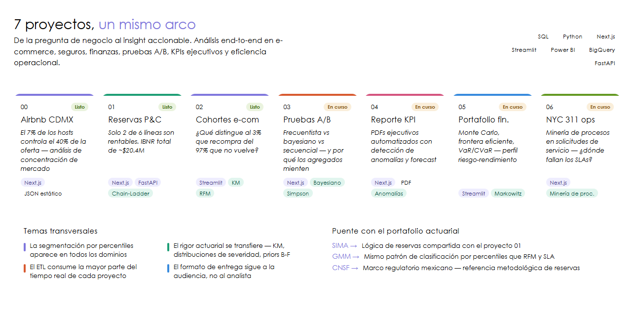
A data analyst’s job is not to produce charts. It is to convert a business question into an informed decision. Every project in this portfolio follows that full arc: a stakeholder has a question, the data exists in some inconvenient format, the analysis produces a finding, and that finding gets delivered in a format the audience can act on.
These 7 projects cover the full arc of data analysis: from business question to actionable insight, applied to domains ranging from e-commerce to insurance. Actuarial training provides statistical rigor (Kaplan-Meier, severity distributions, reserving methods), and DA roles demand complementary tools: fluent SQL, interactive dashboards, storytelling for non-technical audiences, and the ability to move across domains without losing depth.
The connecting thread is methodological: careful ETL, exploratory analysis before any conclusion, segmentation as a recurring tool, and delivery in whatever format the stakeholder needs, whether that is an interactive dashboard, an automated PDF, or a Streamlit app.
The 7 projects
00 - Airbnb CDMX: market analysis
Business question: How is Mexico City’s short-term rental market structured, and how concentrated is supply?
The Inside Airbnb dataset for CDMX contains 27,051 listings across 79 columns. The ETL pipeline cleans prices (arrive as strings with currency symbols), handles nulls, and segments hosts into enterprise vs. casual operators. The central finding: 7% of hosts control 40% of supply. Blueground, Mr. W, and Clau are not individuals sharing their apartment; they are hospitality companies operating at industrial scale. Cuauhtemoc concentrates 46% of listings, while peripheral boroughs like Tlalpan (MXN 2,493 average) show premium pricing with thin supply.
Dashboard built with Next.js and Recharts, static architecture (precomputed JSON, zero backend).
Status: Complete | Live app | GitHub
01 - P&C actuarial reserves: IBNR and loss experience
Business question: Of the 6 lines of business in the portfolio, which are profitable and what is the total IBNR (incurred but not reported) the insurer must reserve?
US insurers are required to file their claims history with regulators in a standardized format called NAIC Schedule P: essentially a table showing, for each accident year, how much has been paid and how much is still outstanding. The challenge is that many claims take years to surface. Medical Malpractice insurance, which covers medical errors like a botched surgery or a missed diagnosis, can produce lawsuits that emerge 5 to 7 years after the incident. Compare that to auto insurance, where you know the damage the same day the accident happens.
Chain-Ladder and Bornhuetter-Ferguson address that problem differently: the first extrapolates historical claim development patterns to project what is still outstanding; the second blends that projection with an industry-wide prior when the insurer’s own data is thin. Both produce an estimate of the IBNR: the money the insurer must set aside today for accidents that have already happened but have not yet been filed as claims.
The most revealing finding: Medical Malpractice shows a loss ratio of ~280%, meaning for every $100 in premiums collected, the insurer paid $280 in claims. That is not a bad year; it is a structural pricing problem. Only Private Passenger Auto and Product Liability are profitable. Total portfolio IBNR is ~$20.4M, concentrated in the lines where claims take the longest to resolve.
Interactive dashboard with Next.js and FastAPI: loss triangle heatmap, IBNR waterfall, frequency-severity and combined ratio trend.
Status: Complete | Live app | GitHub
02 - E-Commerce cohorts: retention, RFM, and LTV
Business question: What differentiates the 3% of Olist customers who repurchase from the 97% who never return?
The Olist dataset has ~99K orders across 9 data files. The finding that reframes everything: only ~3% of customers come back for a second purchase. In a typical e-commerce business that would be a crisis; here it is the reality of the Brazilian market in that period, and it shifts the question from “how well do we retain?” to “what is different about that 3%?”
One technical detail that matters: the dataset has two customer identifier fields, and using the wrong one makes every order look like a new customer, artificially inflating retention numbers. Getting that right is the first step before any analysis is trustworthy.
The analysis builds four views of that 3%: a heatmap showing how many customers from each purchase month returned in the following months; a survival curve tracing how quickly buyers are lost over time; an RFM segmentation (Recency, Frequency, Monetary value) grouping customers by how recently they bought, how often, and how much they spent; and an estimate of the total revenue each segment will generate over their lifetime as a customer.
Streamlit app deployed on Cloud Run with full technical pipeline visible (notebooks converted to HTML embedded in the app).
Status: Complete | Live app | GitHub
03 - A/B Testing: frequentist, Bayesian, and Simpson’s Paradox
Business question: If we run a conversion A/B test, which statistical approach gives us the most reliable answer and why can aggregated results lie?
Imagine a product team wants to know whether changing the checkout button from blue to green increases conversions. They run the experiment for two weeks, and the global result shows the green version wins by 2 percentage points. Do you ship it? That depends on how you answer three questions: is that difference real or is it noise? How much confidence do you need before making the call? And if you split the result by mobile vs desktop users, does green still win in both groups?
The project evaluates that exact situation using three statistical approaches: classic frequentist testing (is the p-value below 0.05?), Bayesian inference with PyMC (what is the probability that B beats A, and by how much?), and sequential monitoring (can you stop early if the answer is already obvious?). The central analysis is Simpson’s Paradox: how a result that looks clear at the aggregate level can reverse completely when you segment by subgroup, a real risk in any product experiment.
Interactive Next.js dashboard for exploring each statistical approach, calculating test power, and visualizing Bayesian convergence.
Status: Complete | Live app | GitHub
04 - Executive KPI Report: automated SaaS metrics
Business question: How to automate monthly executive report generation with anomaly detection and key metric forecasting?
CEOs and VPs do not live in dashboards. They receive a PDF or slide deck once a month. The problem with the manual process: it takes a full day to assemble, the numbers are always slightly stale, and anomalies only get caught if someone happens to be looking at the right chart at the right time. A month with unusually high churn can slip through unnoticed.
This pipeline replaces that process. A single command generates the complete report: calculates the key SaaS metrics (MRR, churn, customer acquisition cost, lifetime value), automatically flags any metric that deviates from its historical trend, forecasts the next quarter, and produces a bilingual PDF ready to send. The analyst spends their time interpreting findings, not copying numbers between spreadsheets.
9 notebooks covering data generation, EDA, anomaly detection, forecasting, report automation, backend architecture, KPI calculations, analytics algorithms, and PDF pipeline. Complementary Next.js dashboard.
Status: Complete | Live app | GitHub
05 - Financial Portfolio: Monte Carlo and efficient frontier
Business question: Given a diversified ETF portfolio, does that diversification actually pay off compared to simply buying the S&P 500?
The dashboard analyzes a real 6-ETF portfolio spanning different asset classes, with live data from Yahoo Finance and the S&P 500 as the benchmark. The central question is simple but uncomfortable: if your diversified portfolio had worse risk-adjusted performance than a single index ETF, diversification cost you money rather than protecting you.
To answer that rigorously, the analysis calculates the Markowitz efficient frontier (the set of portfolios that maximize return for each level of risk), runs Monte Carlo simulations to map the range of plausible future outcomes, and measures risk in multiple ways: VaR (maximum expected loss under normal conditions), CVaR (expected loss in worst-case scenarios), and the Sharpe and Sortino ratios (return per unit of risk). The result is a quantitative answer to whether your asset mix makes mathematical sense.
5 notebooks covering data acquisition, portfolio construction, performance analysis, risk analytics, and Monte Carlo frontier optimization.
Status: Complete | Live app | GitHub
06 - Operational Efficiency: NYC 311, process mining, and SLA
Business question: What inefficiency patterns exist in NYC 311 service requests and where are SLAs systematically violated?
NYC 311 is New York City’s public service complaint system: residents report potholes, noise, rat infestations, building code violations, broken heating, accumulated garbage. Over 30 million records since 2010, spanning 40+ complaint types across 20+ agencies. It is a massive dataset, but what makes it interesting for operational analysis is not the volume — it is what it captures implicitly.
The data records when each complaint was opened and when it was closed, but not the steps in between. Process mining reconstructs those hidden workflows: if a building violation complaint takes 14 days on average but the fastest ones close in 2, the algorithm looks for what the fast resolutions have in common. That surfaces the real bottlenecks, not the reported ones.
What the analysis makes visible that simple averages miss: some agencies have SLA (service level agreement) commitments that are structurally impossible to meet given their complaint volume — not because they are slow, but because the target was set without accounting for actual demand. Response times in certain neighborhoods are systematically slower for identical complaints compared to other areas. Certain complaint types have predictable seasonal spikes that pile up into backlogs when agencies do not adjust capacity. The dashboard makes those patterns navigable by agency, complaint type, neighborhood, and time period.
Next.js dashboard with process flow visualizations, SLA heatmaps, and agency rankings.
Status: Complete | Live app | GitHub
Architecture decisions
The choice of delivery tool is not arbitrary. It depends on three factors: who is the audience, how interactive does the output need to be, and what is the update cycle.
Next.js (projects 00, 01, 03, 04, 06) when the dashboard is a finished product that needs full control over aesthetics, dark mode, mobile responsiveness, and reusable components across projects. The cost is higher: it requires knowledge of React, TypeScript, and a build pipeline. It is justified when the dashboard has a long shelf life or when components are genuinely reused (KPICard, ChartContainer, and ThemeToggle are shared across all Next.js dashboards).
Streamlit (projects 02, 05) when the analysis lives in Python and the priority is moving from notebook to interactive app with minimal overhead. Streamlit is the right choice when the analyst maintaining the app is the same person who wrote the analysis and the Python stack is already established. The notebook-in-Streamlit pattern (converting notebooks to HTML and embedding them as a technical process page) adds portfolio value: the viewer sees the complete code behind every visualization without leaving the app.
Power BI appears in the plan for projects 04 and 06 as a complementary format, aimed at stakeholders who already work in the Microsoft ecosystem and expect drag-and-drop segmentation filters.
The decision between static JSON (Airbnb, zero backend) and FastAPI backend (Olist, Insurance) depends on whether user filters change the underlying computation. If the data fits in memory and aggregations are fixed, static JSON eliminates all infrastructure complexity. If cohort analysis or loss triangles depend on applied filters, the backend is necessary.
Cross-project learnings
After building 7 projects across different domains, the recurring patterns are more instructive than any individual finding.
ETL consumes most of the actual time. In every project, data cleaning and transformation took more time than the analysis itself. Airbnb prices arrive as strings with currency symbols and commas. Olist timestamps need careful parsing to build correct cohorts. NAIC Schedule P data requires cross-table validation before building reliable triangles. NYC 311 data has agency-level inconsistencies in how request types are recorded. The methodology transfers: type validation, explicit null handling, logging of discarded records.
Percentile-based segmentation appears in every domain. Classifying Airbnb hosts as enterprise vs. casual (by listing count), segmenting Olist customers into RFM clusters (by recency, frequency, and monetary value), classifying insurance lines by tail profile, segmenting NYC agencies by SLA compliance. The pattern is identical: define thresholds on a distribution, assign labels, measure differences between groups, make decisions based on the heterogeneity.
Olist’s 3% repurchase rate changes how you frame cohort analysis. When the vast majority of customers are one-time buyers, the question is not “how well do we retain” but “what differentiates those who return.” That reframing applies in insurance (what differentiates policies that renew), in SaaS (what differentiates users who don’t churn), and in any business with high attrition.
Actuarial statistical rigor applies directly to product analytics. Kaplan-Meier is a curve showing what fraction of customers remained active at each point in time, without needing everyone to have left before you can estimate the trend — in insurance it models how many policyholders are still alive; in product analytics, how many users are still buying. Severity distributions describe not just the average transaction amount but the full shape of the distribution: how many customers spend $50, how many spend $500, how many spend $5,000, which is exactly what you need to estimate customer lifetime value without outliers distorting the average. Bornhuetter-Ferguson blends what your current data says with what industry-wide historical experience suggests — useful when you have too few observations to trust your own data alone. The point is not the names. It is that insurance analytics and product analytics solve the same underlying problem: estimating what has not yet happened from what you have already observed.
Connections to the actuarial portfolio
This DA portfolio does not exist in isolation. The actuarial projects in the main portfolio directly complement the work here:
- SIMA (Integrated Actuarial Modeling System) shares reserve calculation logic with project 01, though for life products rather than P&C. The same discount factors and development patterns that appear in the NAIC triangles live as modular functions in SIMA’s engine.
- GMM Explorer connects to the segmentation across this portfolio: defining groups from Major Medical Expenses claim distributions is the same percentile-classification pattern that appears in RFM, host segmentation, and SLA analysis.
- The insurance technical notes (life and property) provide the regulatory reference: the CNSF frameworks governing how reserves are calculated in the Mexican market. Project 01’s methodology is analogous, adapted to the US regulatory context (NAIC).
Reference materials
- Main GitHub repository: Complete source code for all 7 projects, numbered notebooks, SQL queries, ETL pipelines, and deployment configuration.
- Airbnb CDMX (Live app): Next.js dashboard with short-term rental market analysis.
- P&C Actuarial Reserves (Live app): Next.js + FastAPI dashboard with loss triangles and IBNR.
- E-Commerce Cohorts (Live app): Streamlit deployed on Cloud Run with full technical pipeline.
- A/B Testing (Live app): Next.js dashboard with frequentist, Bayesian, and Simpson’s Paradox approaches.
- Executive KPI Report (Live app): Next.js dashboard with automated SaaS metrics.
- Financial Portfolio (Live app): Next.js + FastAPI dashboard with live yfinance data.
- Operational Efficiency (Live app): Next.js dashboard with process mining and SLA analysis.